Data cleaning and preparation (Cont'd)
Stefan Sobernig
November 2nd, 2021
Unit 4
Unit 4
Data cleaning and preparation (Cont'd)
- Missing data
- Data duplicates
- Data outliers (incl. outlier exploration, removal)
Data issues: Running example
Looking into last week's EUROSTAT dataset:
- Accessing/ preprocessing: done
- Data transformation (well, partially covered: e.g. "583034 bde" )
- Missing values? Yes, population for many years missing, even many cities entirely missing
- Duplicate data? E.g. Greater London vs. London City....
- Data outliers? E.g. irregular changes
Data issues: Running example (cont'd)
Question.
What if we want a more complete set of cities?
Another dataset: UN Data
Downloaded dataset as CSV: ./data/UNdata_Export_20171106_004028652.csv
Let's look into this dataset... and think about the following question:
- What is the current population of capitals in Europe?
- What are capitals in Europe? (E.g., what about Bern, Moscow?)
- How can I disambiguate and consolidate data between the different sources?
- How can I reconcile format differences between the Eurostat data and UN city data?
- Which of the typical issues occur?
Data issues: Running example (cont'd)
Issues in the UN data file for instance:
- different format
- No identifiers for cities (different city with the same name, but different types or countries)
- Different identifiers for 'indicators'
- "footnotes" in the CSV file
Missing data (1)
- One or several data objects miss one or several values corresponding to one or several variables (attributes).
- Reasons for missingness, e.g.:
- Structurally or temporarily missing data:
- Not all variables (knowingly) applicable to all data objects.
- Not all variables (knowingly) available at all points in time of data recording (measurement).
- Data-generation processes leading to missingness:
- Missing completely at random (MCAR)
- Missing at random (MAR)
- Not missing at random (MNAR)
- Tactics for dealing with missing data:
- Elimination, filtering
- Imputation: single, multiple
Missing data (2)
Is there an underlying reason for data being missing?
The imagined "process" having produced missing data is independent from the (other) variables in a dataset.
Exemplary "processes":
- Equipment needed for measurement suffered a malfunction or service outage.
- Unplanned termination of data collection.
- Details of data collection (e.g., survey) implies that certain values are missing (e.g., conditional questions in survey)
Generally: The probability of a value being missing is unrelated to the value itself or any other variable in the data set. Therefore, the missing data is said being missing completely at random (MCAR).
Missing data (3)
The imagined "process" having produced missing data is conditional, dependent on the (other) variables in a dataset.
Exemplary "processes":
- Repeated measurement based on some intervention on participants (long term), those not benefiting from the intervention are likely to drop out of the study.
- Demographic profiles may lead to an increased or decreased likelihood that certain data points can be collected or not (e.g., income levels)
Generally: The probability of a value being missing is unrelated to the value itself, but it is associated with other variables in the data set. Therefore, the missing data is said being missing at random (MAR).
Missing data (4)
The imagined "process" having produced missing data is conditional, dependent on the levels of the missing values themselves.
Exemplary "processes":
- Missing product ratings (webshop): Only those making extremely positive or extremely negative product experiences leave ratings at all.
- Missing population counts: City officials fail to report their "official" numbers (up to certain thresholds), because they fear remedies in budget allocation.
- Non-response behaviour (survey): If asking for a certain disease (e.g., which are known to stigmatise patients), patients suffering from that disease are less likely to respond.
Generally: The probability of a value being missing is then related to the (expected) value itself. Therefore, the missing data is said being missing not at random (MNAR).
Missing data (5): Handling missings
- Deletion: Missing data is removed from the dataset for different scopes.
- Objectwise deletion: Any data objects with a value missing from one or several variables is dropped from the dataset.
Notice.
In the case of `urb_cpop1.csv' this would delete all data!
- Pairwise deletion: For various (all) combinations of variables (pairs), data objects are removed when they miss a value from the paired variables.
- In favour: straight forward; if data is MCAR, we reduce the precision (power) of any analysis (=fewer data objects).
- Against: only applicable for minority cases of missing data; typically, MCAR assumption does not hold.
Missing data (6): Handling missings
Single imputation (a.k.a. single substitution):
- Mean imputation for quantitative variables: Substitute the mean of available values for the missing values of a given variable.
- Mode imputation for qualitative variables: Substitute the most common value (mode) for the missing values of a given variable.
- In favour: Allows for complete-case analysis, removes bias only when data is MCAR
- Against: still bias when MAR and MNAR; replacement values are all identical, so the variances end up smaller than in real data.
- Refinements: conditional mean/mode imputation (within homogeneous groups of data objects).
Missing data (7): Handling missings
Single imputation (cont'd)
- Simple imputation techniques suffer from one major limitation, whatever the refinement: They do not reflect the variance in ("real") datasets without missing values.
- Objective: Estimate (interpolate) replacement values with data noise ("error") to it.
- Some examples:
- Regression imputation: a) compute (e.g., linear) regression model over the data, b) used predicted values for the incomplete data objects.
- Last observation carried forward (LOCF): In time-ordered data, take the last observed value for this missing slots.
Missing data (8): Handling missings
Multiple imputation (procedure)
- Starting from the incomplete dataset, create multiple (>1) complete datasets.
- These multiple, imputed datasets are created by replacing the missing values by plausible values.
- Plausible values are computed for each missing value based on a pool of possible values specific for each missing value (hot decks, predictive mean matching)
- The subsequent analysis is then performed for each imputed dataset (e.g., descriptive or inferential statistics).
- The final result (e.g., combined statistic) is then computed ("pooled") from the individual results per imputed dataset.
Main benefit: The individual results for each dataset will differ from each other, and one captures these differences systematically to express the uncertainty in the imagined ("real") dataset.
Missing data (9): Handling missings
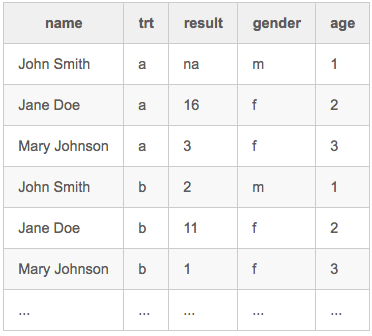
Hot-deck multiple imputation (ex.):

- Requires: Availability of additional, categorical variables as predictors (e.g., gender, age).
Missing data (10): Handling missings
Hot-deck multiple imputation (ex., cont'd):
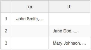
- Form a contingency table based on the predictors, e.g.

- Identify cells holding data objects w/ missing values
- Use the non-missing data objects in the same cell as a pool of "donor" values.
- Draw randomly on "donor" value to impute the missing value (alternative: use a similar donor object).
- Repeat the step foreach cell.
- Repeat the overall process a number of times, to arrive at m > 1 imputed datasets.
Limitation: Restricted to categorical variables as predictors; more generally: "predictive mean matching" (PMM)
Missing data (11)
A small demo on our running example: How can we deal with missing
population values in the Urban Audit data set?
See LOCF applied in this "notebook URL: 05_What_is_the_biggest_European_city_pandas.ipynb
Duplicate data / Deduplication (1)
- A dataset includes data objects (units of observation) that are (almost) duplicates of one another.
- "full" duplicates (observation measurements identical)
- "inconcistent" duplicates (observation measurements differ, on the same identifier/dimensions)
- Data cleaning involves
- detecting and, then,
- removing (and resolving inconsistent) duplicates from the dataset.
- Tackling duplicate data (removal, annotation) is also referred to as deduplication.
Question.
What do you consider common causes for duplicate data?
Have you experienced occurrences of duplicate data in your assignment-2 datasets?
Duplicate data (2)
Two kinds of causes:
- Intra-source duplicates: Data about one data object is entered (inadvertently) multiple times into the same dataset.
- Inter-source duplicates: Combining several datasets, some (all) of which contain (fully or partly overlapping) representations on one and the same data object (observation).
- Detection proceeds similar for both kinds, but the deduplication strategies can differ, e.g.:
- Removal or "unification" for intra-source duplicates.
- Annotation for inter-source duplicates, with duplicate handling left to the data scientists upon data application (e.g., depending on the analysis type).
-->
Duplicate data (2)
Two kinds of causes:
- Intra-source duplicates: Data about one data object is entered (inadvertently, consistently vs. inconsistently) multiple times into the same dataset.
- Inter-source duplicates: Data ends up duplicated after combining several datasets, some (all) of which contain (fully or partly overlapping) representations on one and the same data object (observation).
- Detection proceeds similar for both kinds, but the deduplication strategies can differ, e.g.:
- Removal or "unification" for intra-source duplicates.
- Annotation for inter-source duplicates, with duplicate handling left to the data scientists upon data application (e.g., depending on the analysis type).
Duplicate data (3)
Examples of intra-source duplicates:
- Inadvertent cloning on data entry
- Poor data entry:
- character flipping ("1969" vs. "1996"),
- spelling/case errors, typos ("Vienna" vs. "Viena", "Vienna" vs. "vienna", etc.)
- trained vs. untrained "data clerks"
- non-human sources of duplicates: automated text recognition (e.g., OCR)
- "real" duplicate observations (ie., disambiguating dimension missing in the data), e.g.:
- different kinds of population numbers in the same dataset (estimated vs. as per census)
- two cities named "Vienna"
Duplicate data (4)
Examples of inter-source duplicates:
- Different requirements on entering data (because of different "authorities")
- Different data-entry times (e.g., source years)
- Different data schemata, e.g.:
- name conflicts (variables, attributes)
- data aggregation
- complementary data items on a given data object
Duplicate data (5)
Challenges:
- False negatives: If two or more objects are meant to represent a single one, then the values of the corresponding variables may still differ (inconsistent values).
- False positives: Two or more objects may share values (normalized or not), but still are not duplicates (i.e. should not be removed)
- If the cleaned dataset ends up containing (intended) duplicates, further processing and analysis might be challenging (e.g., misleading grouping or aggregation of values across duplicates).
- Even when duplicates can be detected and inspected in a semi-automated manner, how does detection scale to very large datasets?
--> Inspection and heuristics needed! Deduplication is often an iterative process!
Duplicate data (6a)
Steps in a (prototypical) deduplication procedure include:
- Data preparation:
- schema matching (correspondences between variables/ attributes)
- data transformations (see Unit 3)
- data standardization (e.g. transforming data to all lower case), but also: standardizing data collection
- Search-space reduction: How can we reduce the number of comparisons?
- In a naive approach, the data objects in a dataset have to be compared in a pairwise manner.
- How to to scale duplication detection to even moderately large datasets?
- Comparison-function selection:
- Which techniques for computing similarity/ dissimilarity between pairs of data objects?
- Decision depending on:
- Number of variables for the comparison (1- vs. n-dimensional)
- Type of the variables (quantitative vs. qualitative)
- Definition of similarity/ dissimilarity (or, proximity vs. distance)
Duplicate data (6b)
Steps in a (prototypical) deduplication procedure (cont'd):
- (Manual) Inspection of the candidate duplicates to make a match decision: All pairs of data objects are grouped into either:
- matches ("true positive"): a pair of two data objects represents one single data object.
- non-matches ("true negative"): a pair of two data objects represents two distinct data objects.
- Verification of the quality of duplicate detection (if not ok, start all over from step 2)
- Accuracy
- Scalability
- There is commonly a tradeoff between accuracy and scalability!
Duplicate data (7)
How to scale deduplication? (Hint: numbe of pairwise comparisons: \( (n^2-n)/2 \))
Different strategies (or mixes thereof could be deployed):
- Sorting (intra-source duplicate dedection):
- first sort (n*log(n))
- then run through all records in one scan and check duplicates (n)
- Blocking ("Divide and Conquer")
- Group data objects into disjoint subsets based on maximally discriminating variables ("blocking keys")
- Each block can be checked for duplicates separately (or even better, in parallel)
- Note: this might actually involve sorting!
- Windowing:
- For inter-source duplicate dedection, sort data objects in each dataset according to values by matching variables ("sorting key").
- Slide windows of a certain size over the sorted data records.
- Note: this would be similar to a "sort-merge-join" in Databases
- Use hashing instead of sorting
- etc.
Duplicate data (8): Ex. inter-source duplicates
Example:
Question.
What's the number of inhabitants of 'London'?
What issues can you run into answering these questions?
Candidate issues:
- There might be different interpretations of what 'London' as an entity is (City Area vs. Greater London urban agglomeration area)
- Name ambiguity: there might be several cities called 'London'
- When combining data: There might be several different population numbers from different sources for London.
- Other issues "hiding" actual duplicates, such as language issues ("Londres" vs. "London")
Duplicate data (9): Ex. inter-source duplicates
Candidate tactics:
- Define a trust preference/choices, e.g.: I prefer values from source A to values from source B
- Data aggregation to the rescue, e.g. pich the:
- Maximum value
- Most recent value
- Pick "average" value (mean/median/mode)
- Nota bene: Similar tactics as in missing-data imputation!
Example in Python - Discuss potential issues with Duplicates in city population
data: 05_What_is_the_biggest_European_city_pandas_continued.ipynb
Data outliers (1)
Data outliers are ...
- data objects that have characteristics which are different from the majority of the data objects.
- values of a variable which are unusual with respect to the typical
values of the variable.
- Outliers can be perfectly legitimate and genuine data objects, depending on the
(research, analysis) setting!
- Handling outliers ranges from:
- data removal,
- data substitution (imputation), to
- data analysis being robust against data outliers.
Question.
What approaches could we use to detect outliers in 1-dimensional data?
Data outliers (2): 1-dimensional data
- A common approach of finding outliers in one-dimensional data is to mark as a potential outlier:
- A point that is different from reference point(s) in the data.
- A point that has a certain distance from the selected reference
- point(s) (e.g., median, mean, or "typical" range).
- Conventionally: Mean and standard deviation. Values more than \( x \)
standard deviations from the mean.
- Median and Median Absolute Deviation (MAD): Outliers are values
which are outside the median of the absolute deviations from the
data's median (e.g., three-fold or more).
- Other Alternatives:
- Outliers based on inter-quantile range (IQR): Mark all values as outliers which are outside a certain factor of the inter-quantile range
- Outliers based on percentiles: Mark all values as outliers which are outside a certain percentile range (95%).
(More sophisticated outlier-detection methods and techniques, based on
machine learning and models of data distribution are beyond this
course's scope.)
Data outliers (3): X-fold standard deviation
Mark all values as outliers which are X times the standard deviation away from the mean.
import numpy as np
def xStddevAway(points, x=2):
    mean= np.mean(points)
    stddev=np.std(points)
    abs_dev = np.abs(points - mean)
    return (abs_dev>x*stddev)
Data outliers (4): MAD
The Median Absolute Deviation (MAD) for a univariate dataset \( X_1 \), \( X_2 \), ..., \( X_n \) is defined as the median of the absolute deviations from the data's median:
- \( MAD =median (| X_i - median(X)|) \)
- That is: 1) Compute the residuals (absolute deviations) of all data points from the data's median, 2) take the median of these residuals.
- Advantages:
- The median is a robust descriptor of data (i.e., a descriptor which is not influenced by data outliers itself).
- The median describes data whose (probability) distribution is unknown or is not Gaussian (or, generally, symmetric).
In practice, one could consider a library implementation, such as
pandas MAD.
Data outliers (6): IQR
The inter-quantile-range (IQR) approach marks outliers as the data
points which are \( x \) times the inter-quantile range below the 25%
quantile and/ or above the 75% quantile.
import numpy as np
def interQuantil(points, distance=3):
    q25, q75=np.percentile(points, [25, 75])
    IQ= q75-q25
    minval= q25-distance*IQ
    maxval= q75+distance*IQ
    return (points < minval) | (points > maxval)
Some more information can be found at the Engineering statistic handbook
Data outliers (7): percentiles
Mark all values as outliers which are outside a certain percentile range.
import numpy as np
def percentile_based_outlier(data, threshold=95):
   # Marks all data points which are below the 2.5% quantile or above the 97.5% quantile
    diff = (100 - threshold) / 2.0
    minval, maxval = np.percentile(data, [diff, 100 - diff])
    return (data < minval) | (data > maxval)
Data outliers (8): Examples
l=[1, 2, 3, 3, 4, 4, 4, 5, 5.5, 6, 6, 6.5, 7, 7, 7.5, 8, 9, 12, 52, 90]
>>>print(interQuantil(l,distance=3))
[False False False False False False False False False False False False
 False False False False False False  True  True]
>>>print(percentile_based_outlier(l))
[ True False False False False False False False False False False False
 False False False False False False False  True]
>>>print(xStddevAway(l,x=2))
[False False False False False False False False False False False False
 False False False False False False False  True]
We see that
the inter-quantil approach filters out the values 52 and 90, while the _percentile_based_outlier_ approach filters 1 and 90 and the two stddev from mean approach only 90.
Data preparation and cleaning: Take-away message
- Data Cleansing/Wrangling/Pre-Processing is a bit like a "Jungle Survival Camp"

- Don't dispair: most data is messy and dirty: issues might seem overwhelming in the beginning
- many dangers and issues ahead!
- you have to often use the "machete" to bring data into workable form:
- make assumptions, remove parts of the data, use "rules of thumb"
- you don't get past them by theory alone
- any dataset has different issues
- Remember: at any stage things can go wrong (GIGO!)
... in this lecture and in the notebooks we cannot do more than
providing some "recipes" or examples... which you should learn to
- adapt/generalize and deploy in your future projects.
References
- Pang-Ning Tan, Michael Steinbach, Vipin Kumar (2006): "Introduction to Data Mining", Chapter 2: "Data", Pearson.
- Felix Naumann and Melanie Herschel (2010): An Introduction to Duplicate Detection, Chapter 2, In: Synthesis Lectures on Data Management, Morgan & Claypool Publishers
- Wenfei Fan and Floris Geerts (2012): Foundations of Data Quality Management, Chapter 4, In: Synthesis Lectures on Data Management, Morgan & Claypool Publishers
- Paul D. Allison (2001): Missing Data, In: Sage University Papers, 136, Sage
- Thom Baguley and Mark Andrews (2016): Handling missing data, In: "Modern Statistical Methods for HCI", eds. J. Robertson and M. Kaptein, Springer.
- Leys, C., et al., Detecting outliers: Do not use standard deviation around the mean, use absolute deviation around the median, Journal of Experimental Social Psychology, Volume 49, Issue 4, July 2013, pp. 764-766.
